a What the paper does
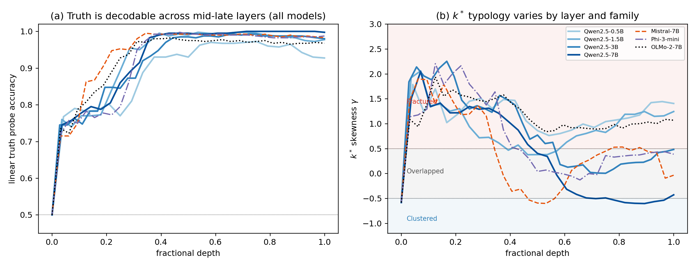
Linear probes read whether a statement is true from a language model's hidden states at ≈0.97–1.00 accuracy. The paper asks what that number hides. It takes the k* distribution (Kotyan, Ueda & Vargas, IEEE TNNLS 2025) — a distortion-free local-neighbourhood statistic that labels a class Clustered, Overlapped, or Fractured from the skewness of its nearest-different-class rank — and applies it to the hidden states of autoregressive LLMs for the first time.
Findings: at matched probe accuracy the local shape of truth differs by model family (Fractured → Clustered on identical inputs); it changes with scale in a layer- and concept-dependent way; and it is fragile across languages, measured by a new Geometric Reliability Coefficient (GRC). Two controlled negative results show this local geometry does not reliably predict probe transfer — the global truth direction travels across models and languages; the local neighbourhood does not follow. Both negatives are reported as such.
- 7 models · 4 familiesQwen2.5 0.5B–14B · Mistral · Phi-3 · OLMo-2
- 8 languagesen es de fr ru zh ar hi · 3 truth concepts
- 2000-sample bootstrap CIspre-registered 14B extension
- controlslabel-permutation · length · random-weight · quantization
b Results
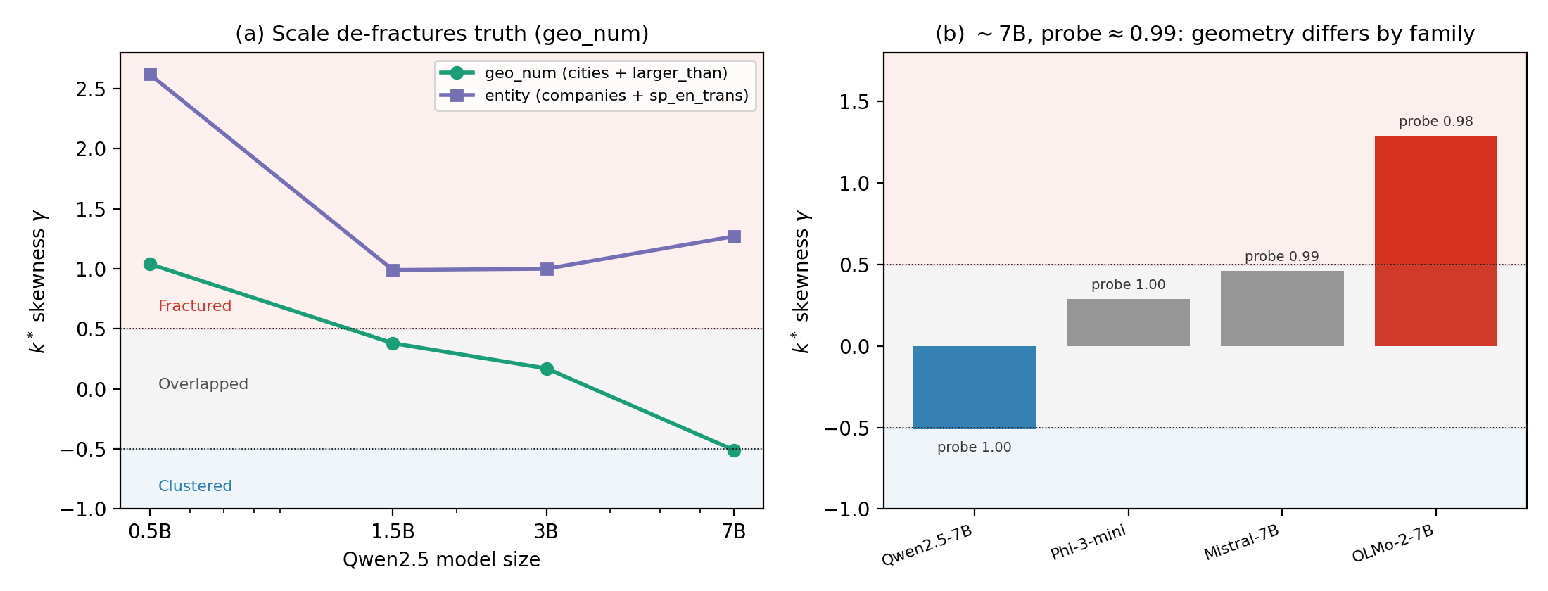
Main result (geo_num concept, read at each model's best-probe layer). Truth is decodable everywhere; the local typology is not the same anywhere.
| model | probe | k* skew γ [95% CI] | typology | GRC |
|---|---|---|---|---|
| Qwen2.5-0.5B | 0.972 | +1.04 [+0.78, +1.32] | Fractured | 0.267 |
| Qwen2.5-1.5B | 0.997 | +0.38 [+0.14, +0.59] | Overlapped | 0.216 |
| Qwen2.5-3B | 0.993 | +0.17 [−0.02, +0.37] | Overlapped | 0.204 |
| Qwen2.5-7B | 1.000 | −0.51 [−0.81, −0.22] | Clustered | 0.096 |
| Qwen2.5-14B | 0.998 | −0.08 [−0.26, +0.10] | Overlapped | — |
| Mistral-7B | 0.995 | +0.46 | Overlapped | 0.256 |
| Phi-3-mini | 0.997 | +0.29 [+0.10, +0.50] | Overlapped | 0.160 |
| OLMo-2-7B | 0.982 | +1.29 [+0.97, +1.63] | Fractured | 0.218 |
notesCIs are 2000-resample bootstrap. Several CIs straddle a ±0.5 boundary, so the robust claim is the family-and-scale ordering, not any single categorical label. Mistral's CI and 14B's GRC were not recomputed in the scale-extension run.
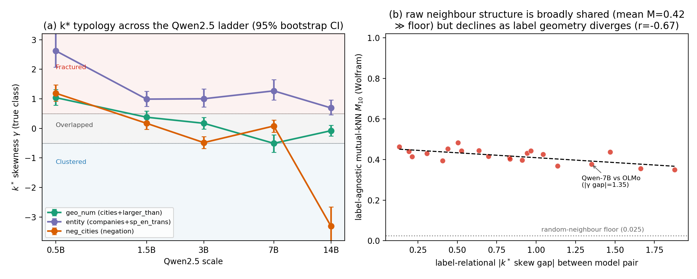
Scale × concept: no single curve describes truth's local geometry. At the probe-peak layer geo_num reverses at 14B; at one matched depth (0.6) the same ladder is monotone (+0.83 → −0.84) — the reversal is a layer-selection effect the paper flags rather than hides.
| concept | 0.5B | 1.5B | 3B | 7B | 14B |
|---|---|---|---|---|---|
| geo_num (cities + larger_than) | +1.04 | +0.38 | +0.17 | −0.51 | −0.08 |
| entity (companies + sp_en_trans) | +2.62 | +0.99 | +1.00 | +1.27 | +0.69 |
| neg_cities (negated facts) | +1.19 | +0.17 | −0.48 | +0.08 | −3.31 |
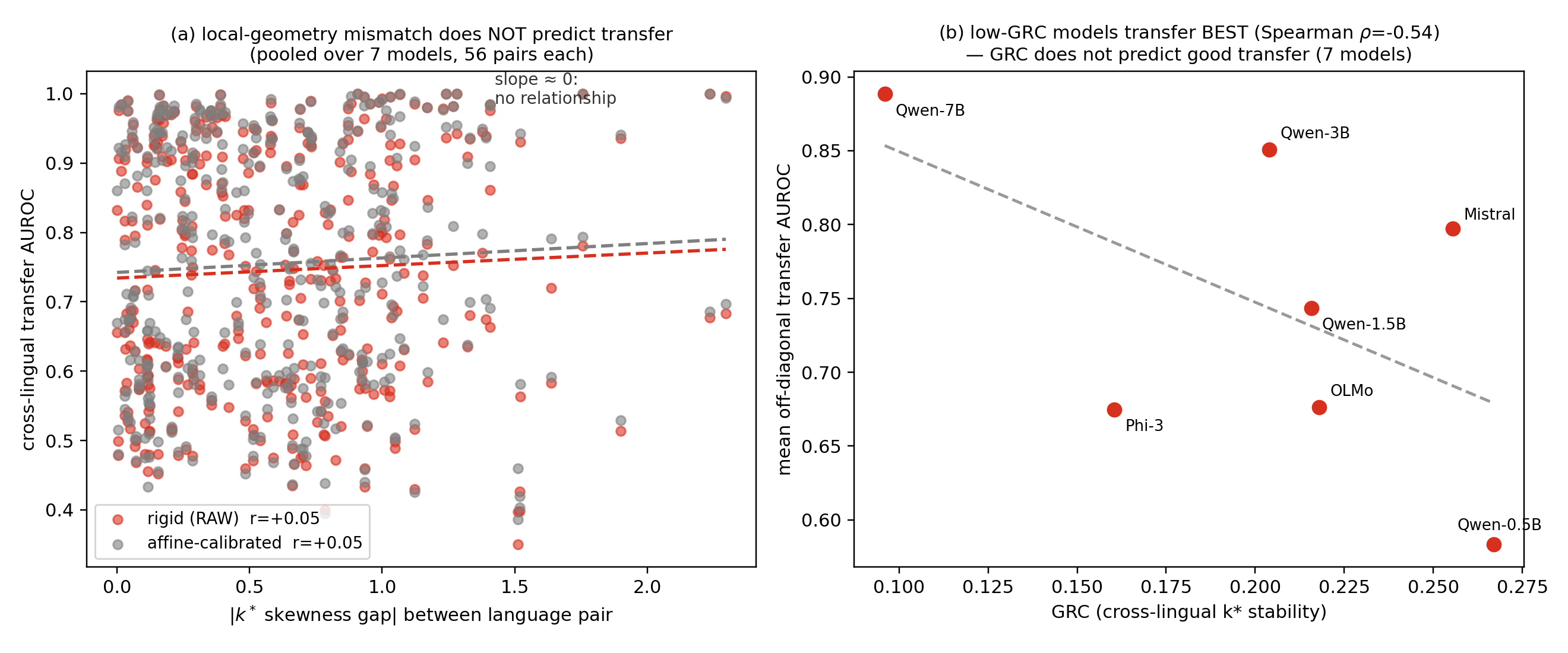
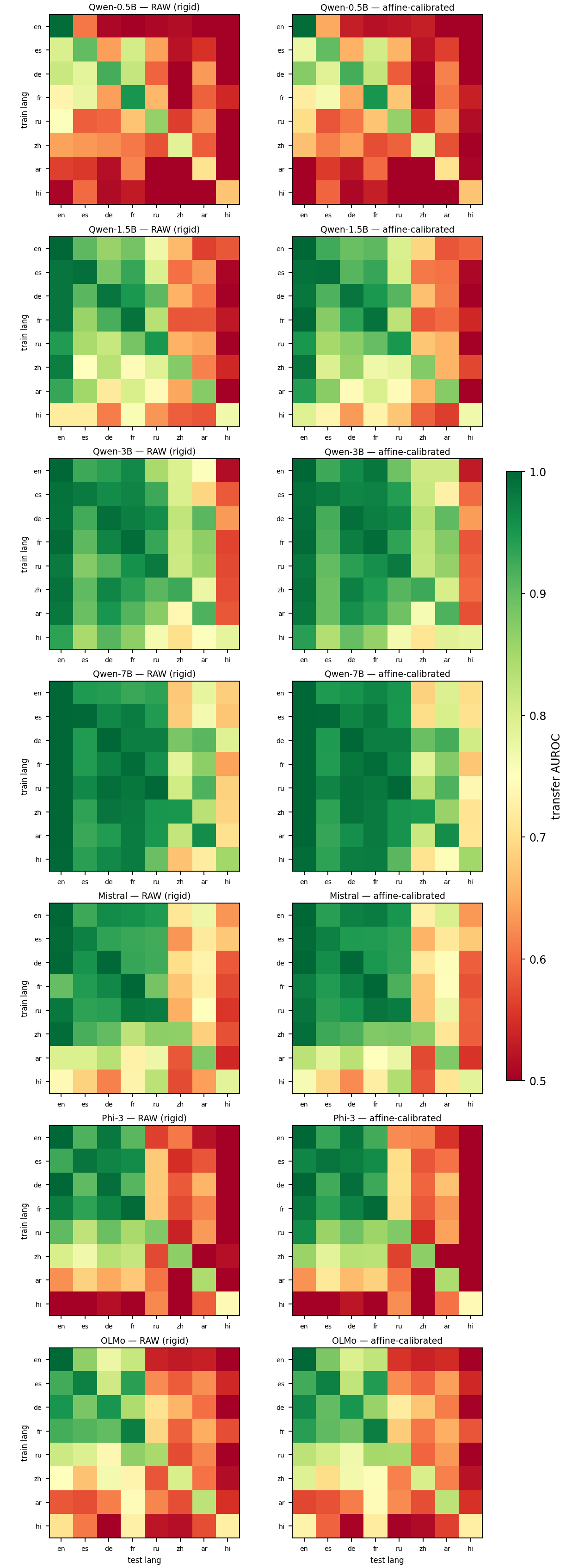
Transfer — the two honest negatives. Cross-model: a learned linear remap recovers the truth direction regardless of local geometry; under a rigid alignment the degradation co-occurs with the k* gap but is outlier-driven and concentrated on the smallest target model. Cross-lingual: token length and script predict transfer; the local geometry does not.
| test | value | note |
|---|---|---|
| cross-model, learned-linear (ridge) | mean 0.996 | k* gap does not predict it (r = +0.19, two-sided Mantel p = 0.51) |
| cross-model, rigid (Procrustes, 64-d PCA) | mean 0.970, worst 0.82 | Pearson r = −0.34 (two-sided Mantel p = 0.029) — but Spearman ρ ≈ 0; six of eight worst pairs share the 0.5B target |
| cross-lingual, 8×8 per model | off-diagonal 0.58 → 0.89 | rises with scale while GRC falls 0.267 → 0.096 |
| per-pair predictor, pooled | k* gap r = +0.05 | null; token-length gap r = −0.55…−0.68 in every model is the consistent predictor |
Controls (the result survives them; the instrument is validated before any LLM number is trusted).
| control | value | conclusion |
|---|---|---|
| label permutation (200 shuffles, 0.5B) | probe 0.975 → 0.499 ± 0.028 | decodability needs true labels (p < 0.001) |
| k* skew vs random-label null | +1.04 vs +1.89 | real labels ≈3 SD less fractured than chance |
| distance metric | euclidean / cosine / cityblock / chebyshev | typology unchanged under all four |
| layer consistency (0.5B) | 24/25 layers | not a cherry-picked layer |
| quantization (Qwen-7B) | bf16 −0.516 vs 4-bit −0.506 | 4-bit extraction does not flip the typology |
| raw neighbour overlap M10 (21 pairs) | 0.35–0.48 ≫ 0.025 floor | family divergence is not unrelated representation spaces (r vs k* gap = −0.67, p = 0.005: a partial, not clean, dissociation) |
c The instrument — kstar.py
The complete measurement core (68 lines, comment-free; the notes between segments stand in for inline comments). It is numerically verified against the paper pipeline and is the file this page lets you download.
The cleaned, comment-free core instrument, numerically verified against the paper pipeline. Four segments, explained between the code instead of inside it.
1 · Nearest-different-class rank kstar_rank
For each sample, rank all others by distance and count how many same-class neighbours appear before the first different-class one. Supports euclidean / cosine / cityblock / chebyshev; the result depends only on neighbour ranks, not absolute distances.
import numpy as np

def kstar_rank(X, y, metric='euclidean', standardize=False):
    X = np.asarray(X, dtype=np.float64)
    y = np.asarray(y)
    if standardize:
        X = (X - X.mean(0, keepdims=True)) / (X.std(0, keepdims=True) + 1e-08)
    if metric == 'cosine':
        Xn = X / (np.linalg.norm(X, axis=1, keepdims=True) + 1e-12)
        D = 1.0 - Xn @ Xn.T
    elif metric in ('cityblock', 'l1'):
        D = np.abs(X[:, None, :] - X[None, :, :]).sum(-1)
    elif metric in ('chebyshev', 'linf'):
        D = np.abs(X[:, None, :] - X[None, :, :]).max(-1)
    else:
        sq = (X * X).sum(1)
        D = np.sqrt(np.maximum(sq[:, None] + sq[None, :] - 2 * X @ X.T, 0.0))
    np.fill_diagonal(D, np.inf)
    order = np.argsort(D, axis=1)
    diff = y[order] != y[:, None]
    kstar = diff.argmax(axis=1)
    has_diff = diff.any(axis=1)
    same_counts = (y[:, None] == y[None, :]).sum(1) - 1
    return np.where(has_diff, kstar, same_counts).astype(int)
2 · Class-size normalisation and typology kstar_normalized, typology_by_class
Divide by the sample's own class cardinality, then label each class by the Fisher–Pearson skewness of its normalised distribution — Fractured (γ > 0.5), Overlapped (|γ| ≤ 0.5), Clustered (γ < −0.5), cut-offs unchanged from the original method.
def _skew_pop(v):
    v = np.asarray(v, dtype=np.float64)
    sd = v.std()
    if sd == 0:
        return 0.0
    return float(((v - v.mean()) ** 3).mean() / sd ** 3)

def kstar_normalized(raw, y):
    y = np.asarray(y)
    out = np.empty(len(raw), dtype=np.float64)
    for c in np.unique(y):
        m = y == c
        out[m] = raw[m] / max(int(m.sum()), 1)
    return out

def typology_by_class(norm_kstar, y):
    y = np.asarray(y)
    res = {}
    for c in np.unique(y):
        v = norm_kstar[y == c]
        g = _skew_pop(v)
        label = 'Fractured' if g > 0.5 else 'Clustered' if g < -0.5 else 'Overlapped'
        res[int(c)] = {'label': label, 'skewness': g, 'mean': float(v.mean()), 'std': float(v.std()), 'n': int(len(v))}
    return res
3 · Uncertainty gamma_bootstrap_ci
Third moments are noisy at small n, so every reported skewness carries a 2000-resample bootstrap 95% CI.
def gamma_bootstrap_ci(norm_kstar, y, cls, n_boot=2000, seed=0):
    v = np.asarray(norm_kstar)[np.asarray(y) == cls]
    rng = np.random.default_rng(seed)
    n = len(v)
    boots = [_skew_pop(v[rng.integers(0, n, n)]) for _ in range(n_boot)]
    return (float(np.percentile(boots, 2.5)), float(np.percentile(boots, 97.5)))
4 · Cross-lingual stability grc_spearman
GRC = mean pairwise Spearman correlation of per-item normalised k* across languages — rank correlation because k* is itself a rank.
def grc_spearman(norm_kstar_by_lang):
    from scipy.stats import spearmanr
    langs = list(norm_kstar_by_lang)
    vals, pairs = ([], [])
    for a in range(len(langs)):
        for b in range(a + 1, len(langs)):
            r, _ = spearmanr(norm_kstar_by_lang[langs[a]], norm_kstar_by_lang[langs[b]])
            r = 0.0 if np.isnan(r) else float(r)
            vals.append(r)
            pairs.append((langs[a], langs[b], round(r, 3)))
    return {'grc': float(np.mean(vals)) if vals else 0.0, 'pairs': pairs}
d Verify it yourself
The instrument is validated on synthetic data with known geometry before any LLM number is trusted. The check below builds three 2-D fixtures — interleaved tight sub-blobs (locally pure → Clustered), two moderately separated Gaussians (Overlapped, the boundary case by construction), and fully interpenetrating Gaussians (Fractured) — and labels them with the exact code above. Needs only numpy and scipy:
pip install numpy scipy
python synthetic_check.py   # with kstar.py in the same folder
import numpy as np
from kstar import kstar_rank, kstar_normalized, typology_by_class
N = 148
def make(kind, rng):
if kind == "clustered":
c = np.array([[i * 2.0, 0] for i in range(8)])
a = np.concatenate([rng.normal(c[i], 0.35, (N // 4, 2)) for i in [0, 2, 4, 6]])
b = np.concatenate([rng.normal(c[i], 0.35, (N // 4, 2)) for i in [1, 3, 5, 7]])
elif kind == "overlapped":
a = rng.normal([0, 0], 1.0, (N, 2))
b = rng.normal([3, 0], 1.0, (N, 2))
else:
a = rng.normal([0, 0], 1.0, (N, 2))
b = rng.normal([0, 0], 1.0, (N, 2))
return np.vstack([a, b]), np.array([1] * len(a) + [0] * len(b))
def band(g):
return "Fractured" if g > 0.5 else "Clustered" if g < -0.5 else "Overlapped"
for kind in ["clustered", "overlapped", "fractured"]:
skews = []
for seed in range(10):
X, y = make(kind, np.random.default_rng(seed))
t = typology_by_class(kstar_normalized(kstar_rank(X, y), y), y)
skews.append(np.mean([t[c]["skewness"] for c in t]))
med = float(np.median(skews))
print(f"{kind:<11} median skew over 10 draws {med:+.2f} -> {band(med)}")Output (deterministic):
clustered   median skew over 10 draws -2.02  ->  Clustered
overlapped  median skew over 10 draws +0.45  ->  Overlapped
fractured   median skew over 10 draws +1.97  ->  Fractured
e Reproducibility & status
- status
- Manuscript, 2026 — under submission preparation; arXiv link will replace the badge above.
- available now
- kstar.py (the instrument) and synthetic_check.py (its validation), both runnable as-is.
- with the paper
- The full extraction-and-analysis pipeline (activation caching, probes, transfer matrices, bootstrap and Mantel tests), per-run result JSONs, and the timestamped pre-registration of the 14B extension.
- honesty
- The two transfer results are negatives and are reported as negatives; the rigid-alignment association is additionally flagged as outlier-driven (Spearman ρ ≈ 0) and entangled with target capacity.